Part 2: Advanced Image Denoising: Innovations and Cutting-Edge Approaches

In continuation with the previous Blog- Image Denoising: Techniques, Challenges, and Solutions , we look into Transformed domain denoising methods.

Transform Domain Filtering in image denoising:

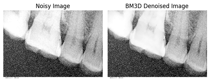
Transform domain filtering is different from the spatial domain in the sense they transform the noisy image to another domain and then denoising methods are applied on it. In this blog let us look into briefly into one such method of BM3D (Link)

Block-Matching and 3D filtering (BM3D) is an advanced denoising algorithm widely used in image processing. It’s known for its remarkable ability to effectively reduce noise while preserving image details and textures. BM3D aims to reduce noise in images by exploiting similar patterns and structures present in different image blocks.

Block Matching:

· Block Matching: BM3D divides the image into overlapping blocks and searches for similar blocks within a search window.

· Grouping Similar Blocks: Blocks that exhibit similar patterns or structures are grouped together.

3D Collaborative Filtering:

· Collaborative Filtering: Similar blocks are stacked into 3D groups (a 3D array) based on their similarity.

· Transform Domain: These 3D groups are transformed into a transform domain (like the Discrete Cosine Transform — DCT).

Denoising Steps:

First Step (Collaborative Filtering):

· Collaborative Wiener Filtering: Wiener filtering is applied to each group in the transform domain.

· Transform Inverse: The processed 3D groups are transformed back to the spatial domain.

Second Step (Aggregation):

· Aggregation: Processed blocks are aggregated, weighting and combining information from overlapping blocks to generate the final denoised image.

· Final Output: The aggregated information is used to construct the denoised image.

Advantages of BM3D:

· High Denoising Performance: BM3D achieves impressive denoising performance, effectively reducing various types of noise.

· Texture Preservation: It preserves image textures and fine details, even in noisy environments.

· Adaptive Nature: BM3D adapts to different noise levels and image characteristics, providing robust denoising across various scenarios.

Applications:

Image Denoising: BM3D is extensively used for denoising tasks in various domains, including medical imaging, photography, and more.

Block-Matching and 3D filtering (BM3D) stands as a benchmark denoising technique due to its ability to effectively reduce noise while preserving image details. Its capacity to handle various noise types and preserve textures makes it a prominent choice in image processing applications, particularly when high-quality denoising is required.

import cv2
import numpy as np
import matplotlib.pyplot as plt

# Load an image
image = cv2.imread('Dataset/1.jpg', cv2.IMREAD_GRAYSCALE) # Load as grayscale

# Add Gaussian noise to the image
def add_gaussian_noise(image):
mean = 0
std_dev = 1
noise = np.random.normal(mean, std_dev, image.shape).astype(np.uint8)
noisy_image = cv2.add(image, noise)
return noisy_image

noisy_image = add_gaussian_noise(image)

# BM3D Denoising (Simplified Example)
bm3d_denoised_image = cv2.fastNlMeansDenoising(noisy_image, None, h=10, templateWindowSize=7, searchWindowSize=21)

# Display the original noisy image and BM3D denoised image
titles = ['Noisy Image', 'BM3D Denoised Image']
images = [noisy_image, bm3d_denoised_image]

for i in range(len(images)):
plt.subplot(1, 2, i + 1)
plt.imshow(images[i], cmap='gray')
plt.title(titles[i])
plt.axis('off')

plt.tight_layout()
plt.show()

CNN Autoencoder for Denoising

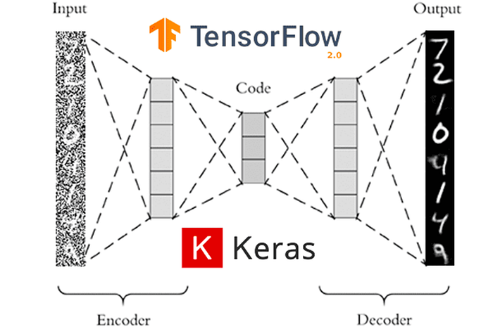
An autoencoder is a type of neural network architecture used in unsupervised learning, especially for tasks like dimensionality reduction, data compression, and, in the context of image processing, image denoising. It consists of an encoder and a decoder, which work together to reconstruct input data, effectively learning to represent the input in a lower-dimensional space.

Components of an Autoencoder:

Encoder:

The encoder takes the input data and compresses it into a latent space representation, typically of lower dimensionality.

It applies a series of transformational layers (convolutional, pooling, etc.) that reduce the input data into a compressed representation.

Decoder:

The decoder receives the compressed representation from the encoder and reconstructs the original input data from this representation.

It applies transformations that upsample or deconvolve the encoded representation back to the original input space.

Autoencoder for Denoising:

An autoencoder can be trained for denoising by taking noisy images as input and the corresponding clean (non-noisy) images as the target output. The model learns to encode and decode the noisy images in a way that minimizes the difference between the decoded output and the clean images.

Training Process for Denoising:

· Dataset Preparation: Collect pairs of noisy images and corresponding clean images.

· Model Architecture: Design an autoencoder architecture consisting of an encoder and decoder.

· Training Setup: Train the autoencoder on the pairs of noisy and clean images.

· Loss Function: Use a loss function (such as Mean Squared Error) that measures the difference between the reconstructed output and the clean image.

· Training Procedure: Optimize the network’s weights to minimize this difference through backpropagation and gradient descent.

Advantages of Autoencoder for Denoising:

· Unsupervised Learning: Autoencoders can learn efficient representations without requiring labeled data, making them suitable for unsupervised denoising tasks.

· Learned Representations: The compressed latent space learned by the encoder often captures meaningful features and structures, aiding in denoising.

· Adaptability: Autoencoders can adapt to different noise levels and patterns, learning to reconstruct clean images from various noisy inputs.

Autoencoders are powerful tools for image denoising, leveraging their ability to learn compressed representations and reconstruct clean images from noisy inputs. By training an autoencoder on pairs of noisy and clean images, it can effectively learn to denoise images, capturing essential features while removing noise. The architecture and training process can be adjusted and optimized to suit different datasets and denoising requirements.

Autoencoder for Denoising Link

from keras.preprocessing import image
import os
train_images = sorted(os.listdir('Dataset/'))

train_image = []
for im in train_images:
img = image.load_img('Dataset/'+ im, target_size=(64,64), color_mode= 'grayscale')
img = image.img_to_array(img)
img = img/255
train_image.append(img)
train_df = np.array(train_image)

import matplotlib.pyplot as plt

def show_img(dataset):
f, ax = plt.subplots(1,5)
f.set_size_inches(40, 20)
for i in range(5,10):
ax[i-5].imshow(dataset[i].reshape(64,64), cmap='gray')
plt.show()

def add_gaussian_noise(image):
mean = 0
std_dev = 1
noise = np.random.normal(mean, std_dev, image.shape) #.astype(np.uint8)
noisy_image = image + noise.reshape(image.shape)*0.05
return noisy_image

noised_df= []

for img in train_df:
noisy= add_gaussian_noise(img)
noised_df.append(noisy)

noised_df= np.array(noised_df)

# Sample Dataset
xnoised= noised_df[0:100]
xtest= noised_df[100:]

from keras.models import Sequential, Model
from keras.layers import Dense, Conv2D, MaxPooling2D,MaxPool2D ,UpSampling2D, Flatten, Input
from keras.optimizers import SGD, Adam, Adadelta, Adagrad
from keras import backend as K

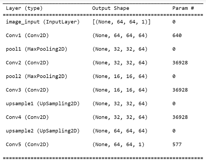
def autoencoder():

input_img = Input(shape=(64,64,1), name='image_input')

#enoder
x = Conv2D(64, (3,3), activation='relu', padding='same', name='Conv1')(input_img)
x = MaxPooling2D((2,2), padding='same', name='pool1')(x)
x = Conv2D(64, (3,3), activation='relu', padding='same', name='Conv2')(x)
x = MaxPooling2D((2,2), padding='same', name='pool2')(x)

#decoder
x = Conv2D(64, (3,3), activation='relu', padding='same', name='Conv3')(x)
x = UpSampling2D((2,2), name='upsample1')(x)
x = Conv2D(64, (3,3), activation='relu', padding='same', name='Conv4')(x)
x = UpSampling2D((2,2), name='upsample2')(x)
x = Conv2D(1, (3,3), activation='sigmoid', padding='same', name='Conv5')(x)

#model
autoencoder = Model(inputs=input_img, outputs=x)
autoencoder.compile(optimizer='adam', loss='binary_crossentropy')

return autoencoder

model= autoencoder()

import tensorflow as tf
from tensorflow.keras.callbacks import EarlyStopping

with tf.device('/device:CPU:0'):
early_stopping = EarlyStopping(monitor='val_loss', min_delta=0, patience=10, verbose=1, mode='auto')
model.fit(xnoised, xnoised, epochs=40, batch_size=10, validation_data=(xtest, xtest), callbacks=[early_stopping])

import cv2

pred= model.predict(xtest[:5])
def plot_predictions(y_true, y_pred):
f, ax = plt.subplots(4, 5)
f.set_size_inches(10.5,7.5)
for i in range(5):
ax[0][i].imshow(np.reshape(xtrain[i], (64,64)), aspect='auto', cmap='gray')
ax[1][i].imshow(np.reshape(y_true[i], (64,64)), aspect='auto', cmap='gray')
ax[2][i].imshow(np.reshape(y_pred[i], (64,64)), aspect='auto', cmap='gray')
ax[3][i].imshow(cv2.medianBlur(xtrain[i], (5)), aspect='auto', cmap='gray')

plt.tight_layout()
plot_predictions(xtest[:5], pred[:5])

Performance Metrics

Most common metrics used to determine the level of noise in the data include

1. Peak Signal to Noise Ratio (PSNR)

2. Structural Similarity Index (SSIM)

Peak Signal to Noise Ratio: It is the ratio of maximum power of a signal to the power of corrupting noise that affects the visual representation. It is represented in logarithmic decibel scale.

Where MSE (Mean Square Error) is given by

Where

1. f represents the matrix data of our original image.
2. g represents the matrix data of our degraded image in question.
3. m represents the numbers of rows of pixels of the images and i represents the index of that row.
4. n represents the number of columns of pixels of the image and j represents the index of that column.
5. MAXf is the maximum signal value that exists in our original “known to be good” image.

Higher the PSNR, the image reconstructed after denoising as a better match to the original image for the algorithm used. This is because the MSE is minimized to maximize PSNR and error between original and reconstructed is reduced as a result.

Structural Similarity Index Measure (SSIM):

It is the measurement of prediction of image quality based on reference as initial distortion free original image. It takes into account 3 components of the image i.e. Luminance (l), contrast ( c ), structure (s). It is different from PSNR in terms of using absolute errors instead of using squared error.

The SSIM formula is calculated using the following components:

Luminance Comparison (l):

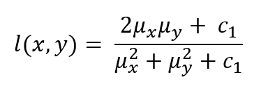
where c1 is a small constant to prevent division by zero.

Contrast Comparison ( c ):

where c2 is another small constant.

Structure Comparison (s):

where c3 is a small constant.

Combined SSIM:

When α,β,γ are 1 then below formula is obtained:

Where

1. μ_x pixel sample mean of x
2. μ_y pixel sample mean of y
3. σ_x² variance of x
4. σ_y² variance of y
5. σ_xy covariance of x and y
6. c_1,c_2 small constants

The SSIM index ranges between -1 and 1, where 1 indicates perfect similarity between the two images.

Recommended Further Study

Other advanced algorithms from that of Autoencoders for denoising that are recommended to be studied for latest information in Image Denoising algorithm space include:

1. CBDNet — Convolutional Blind Denoising Network

2. PRIDNet — Pyramid Real Image Denoising Network

3. RIDNet — Residual Image Denoising Network

Discover cutting-edge innovations in image denoising techniques! Explore advanced data science services that elevate your image processing projects. Contact us for expert support!

AUTHOR - FOLLOW
Aravind Madan Mohan
Data Scientist, Tredence Inc.